Le formulaire complet de mathématiques

Les propriétés des fractions

Opérations élémentaires

Multiplication

Multiplier des fractions entre elles revient à multiplier tous les numérateurs (resp. tous les dénominateurs) entre eux.

Division

Diviser par une fraction revient à multiplier par son inverse.

Addition / soustraction

Additionner (resp. soustraire) des fractions entre elles nécessitent de les mettre sous un dénominateur commun.

Propriétés

Produit en croix

Rapport entre les sommes des numérateurs et dénominateurs respectifs

Les mêmes relations sont possibles en remplaçant tous les \( (+) \) par des \( (-) \).

Rapport entre les sommes et les différences respectives

Addition des numérateurs et dénominateurs entre eux

La même relation est possible en remplaçant le \( (+) \) par un \( (-) \).

1. Généralisation

   De manière générale, avec une série de \(n \) numérateurs et de \(m \) dénominateurs :

   $$ \forall F \in \mathbb{Q}, \enspace \forall (a, c, e ...) \in \hspace{0.04em} \mathbb{N}^n, \enspace (b, d, f...) \in \hspace{0.04em} \mathbb{N}^m, \enspace \ \Bigl \{ (b \textcolor{rgb(118 139 240)}{\pm} d \textcolor{rgb(93 183 129)}{\pm} f \textcolor{rgb(232 124 124)}{\pm} ...) \Bigr \} \ \neq 0, $$
   $$ F = \frac{a}{b} = \frac{c}{d} = \frac{e}{f} = \ ... \ \Longrightarrow F = \frac{a \textcolor{rgb(118 139 240)}{\pm} c \textcolor{rgb(93 183 129)}{\pm} e \textcolor{rgb(232 124 124)}{\pm} \ ...}{b \textcolor{rgb(118 139 240)}{\pm} d \textcolor{rgb(93 183 129)}{\pm} f \textcolor{rgb(232 124 124)}{\pm} \ ...}$$
   $$ (\text{avec les signes de même couleurs étant les mêmes}) $$

Les propriétés des puissances de x (pour des exposants naturels)

Soient \( n\in \mathbb{N}\) un entier naturel et \( x \in \mathbb{R}\) un réel.

On appelle \(x^n\) un nombre \(x\) multiplié \(n\) fois par lui-même :

Produit/quotient de puissances (de même base)

Nombre élevé à la puissance zéro

Inverse d'une puissance

Puissance d'un produit/quotient

Puissance d'une puissance

Le binôme de Newton \(: (a + b)^n \)

Le binôme de Newton nous dit que :

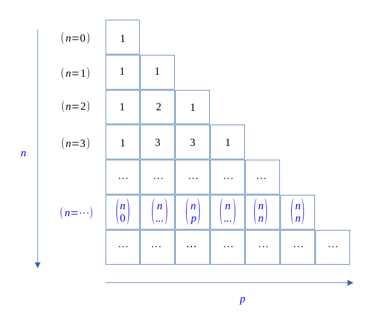
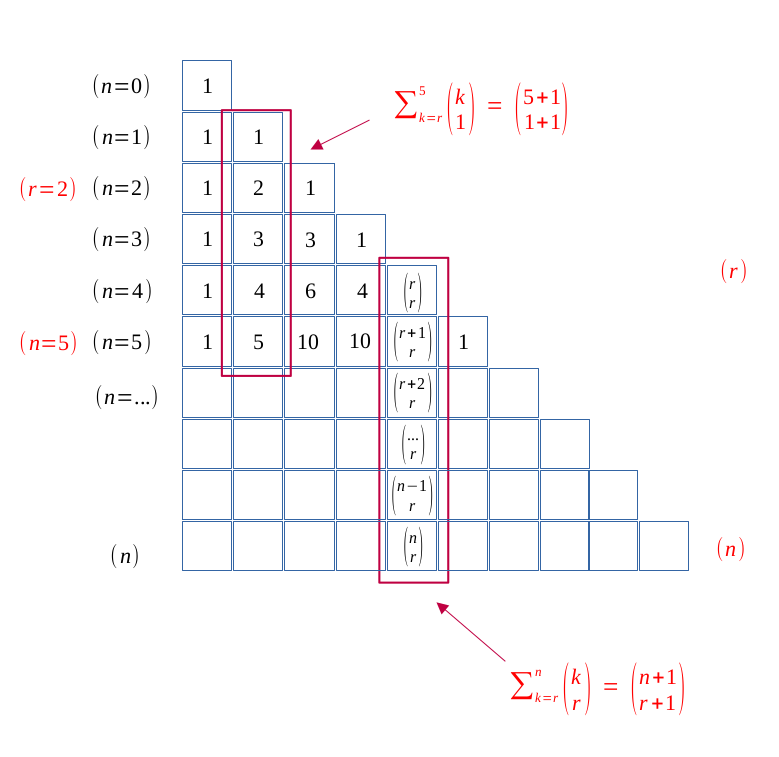
On peut utiliser le triangle de Pascal pour trouver les coefficients binomiaux \(\binom{n}{p}\).

L'identité géométrique

On appelle identité géométrique, ou formule de Bernoulli , l'expression suivante :

Les propriétés du binôme \(: \binom{n}{p}\)

Soient \((p,n) \in \hspace{0.04em}\mathbb{N}^2 \) deux entiers naturels avec \( p \leqslant n \).

On appelle \(\binom{n}{p} \) ("\( p \) parmi \( n \)") le nombre de façons de prendre \( p \) éléments parmi \( n \) éléments d'un ensemble.

On l'appelle aussi le binôme, il répond à la formule suivante :

"0 parmi n" / "n parmi n"

"1 parmi n"

Symétrie

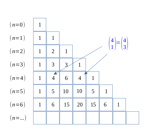
Formule du pion

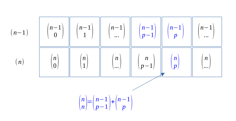
Formule de Pascal

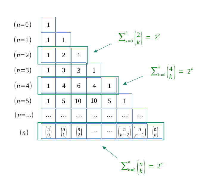
Somme horizontale de 0 à n

Somme verticale de r à n

Les formules de combinatoire et dénombrement

Toutes les formules qui vont suivre auront toujours deux cas :

• sans répétition
• avec répétition : dans ce cas, il y aura une barre au-dessus pour signifier "avec répétition"

  Par exemple, si on note les arrangements sans répétition \(A_n\), on notera \(\overline{A_n}\) ceux avec répétition possible.

Permutations

Le nombre de permutations des éléments d'un ensemble (sans répétition)

Pour tout ensemble \(E\) de \(n\) éléments, le nombre de permutations possibles sans répétition vaut :

Le nombre de permutations des éléments d'un ensemble (avec répétition)

Pour tout ensemble \(E = \{e_1, e_2, e_3, \ ..., \ e_n \}\) avec \(k_1, k_2, k_3, ...,k_{n}\) le nombre d'occurrences de chaque élément, le nombre de permutations possibles vaut :

Arrangements (avec ordre)

Le nombre d'arrangements des éléments d'un ensemble (sans répétition)

Le nombre d'arrangements sans répétition de \(p\) éléments pris dans un ensemble de \(n\) éléments vaut :

Le nombre d'arrangements des éléments d'un ensemble (avec répétition)

Le nombre d'arrangements avec répétition de \(p\) éléments pris dans un ensemble de \(n\) éléments vaut :

Combinaisons (sans ordre)

Le nombre de façons de prendre des éléments distincts d'un ensemble (sans répétition)

Le nombre de façons de prendre \(p\) éléments (distincts et sans répétition) dans un ensemble de \(n\) éléments vaut :

(\(\Longrightarrow\) voir les propriétés du binôme )

Le nombre de façons de prendre des éléments distincts d'un ensemble (avec répétition)

Le nombre de façons de prendre \(p\) éléments (distincts et avec répétition) dans un ensemble de \(n\) éléments vaut :

Le nombre de parties possibles d'un ensemble

Le nombre de parties possibles d'un ensemble \(E = \{e_1, e_2, e_3, \ ..., e_n\}\), c'est-à-dire :

vaut :

Les propriétés des matrices

Pour ce qui suivre, il est important de poser les définitions suivantes :

1. Opérations sur les matrices
   1. Addition de matrices

      Soient deux matrices \((A,B) \in \hspace{0.03em} \mathcal{M}_{n,p} (\mathbb{K})^2\) de même taille.

      $$ \forall (i, j) \in [\![1, n]\!] \times [\![1, p]\!],$$
      $$(A + B)_{i,j} = a_{i,j} + b_{i,j} $$

      Autrement dit, on additionne chaque élément de la matrice de gauche avec l'élément de même position de celle de droite :

      $$ A + B = \begin{pmatrix} a_{1,1} & a_{1,2} & a_{1,3} & \dots & a_{1, p} \\ a_{2,1} & a_{2,2} & a_{2,3} & \dots & a_{2, p} \\ \hspace{0.5em} \vdots & \hspace{0.5em} \vdots & \hspace{0.5em} \vdots & \ddots & \hspace{0.5em} \vdots \\ a_{n,1} & a_{n,2} & a_{n,3} & \dots & a_{n, p} \end{pmatrix} + \begin{pmatrix} b_{1,1} & b_{1,2} & b_{1,3} & \dots & b_{1, p} \\ b_{2,1} & b_{2,2} & b_{2,3} & \dots & b_{2, p} \\ \hspace{0.5em} \vdots & \hspace{0.5em} \vdots & \hspace{0.5em} \vdots & \ddots & \hspace{0.5em} \vdots \\ b_{n,1} & b_{n,2} & b_{n,3} & \dots & b_{n, p} \end{pmatrix} $$
      $$ A + B = \begin{pmatrix} a_{1,1} + b_{1,1} & a_{1,2} + b_{1,2} & a_{1,3} + b_{1,3} & \dots & a_{1, p} + b_{1, p} \\ a_{2,1} + b_{2,1} & a_{2,2} + b_{2,2} & a_{2,3} + b_{2,3} & \dots & a_{2, p} + b_{2,p} \\ \hspace{2em} \vdots & \hspace{2em} \vdots & \hspace{2em} \vdots & \ddots & \hspace{2em} \vdots \\ a_{n,1} + b_{n,1} & a_{n,2} + b_{n,2} & a_{n,3} + b_{n,3} & \dots & a_{n, p} + b_{n,p} \end{pmatrix} $$
   2. Produit matriciel

      Soient deux matrices \(A \in \hspace{0.03em} \mathcal{M}_{n,p} (\mathbb{K})\) et \(B \in \hspace{0.03em} \mathcal{M}_{p,q} (\mathbb{K})\).

      Pour multiplier deux matrices, on a besoin que le matrice de gauche ait le même nombre de colonnes que le nombre de lignes de la matrice de droite (ici \(p\)). Le résultat est une matrice \(AB \in \hspace{0.03em} \mathcal{M}_{n,q} (\mathbb{K})\), donc avec \(n\) lignes et \(q\) colonnes.

      $$ \forall (i, j) \in [\![1, n]\!] \times [\![1, q]\!],$$
      $$(A \times B)_{i,j} = \sum_{k = 1}^p a_{i,k} \times b_{k,j} $$

      Par exemple :

      $$ A \times B = \begin{pmatrix} a_{1,1} & a_{1,2} & a_{1,3} & \dots & a_{1, p} \\ a_{2,1} & a_{2,2} & a_{2,3} & \dots & a_{2, p} \\ \hspace{0.5em} \vdots & \hspace{0.5em} \vdots & \hspace{0.5em} \vdots & \ddots & \hspace{0.5em} \vdots \\ a_{n,1} & a_{n,2} & a_{n,3} & \dots & a_{n, p} \end{pmatrix} \times \begin{pmatrix} b_{1,1} & b_{1,2} & b_{1,3} & \dots & b_{1, q} \\ b_{2,1} & b_{2,2} & b_{2,3} & \dots & b_{2, q} \\ \hspace{0.5em} \vdots & \hspace{0.5em} \vdots & \hspace{0.5em} \vdots & \ddots & \hspace{0.5em} \vdots \\ b_{p,1} & b_{p,2} & b_{p,3} & \dots & b_{p, q} \end{pmatrix} $$
      $$ A \times B = \begin{pmatrix} \Bigl[a_{1,1} b_{1,1} + a_{1,2} b_{2,1} \ + \ ... \ + \ a_{1,p} b_{p,1} \Bigr] & \Bigl[a_{1,1} b_{1,2} + a_{1,2} b_{2,2} \ + \ ... \ + \ a_{1,p} b_{p,2}\Bigr] & \hspace{1em} \dots \dots \dots \hspace{1em} & \Bigl[a_{1,1} b_{1,q} + a_{1,2} b_{2,q} \ + \ ... \ + \ a_{1,p} b_{p,q}\Bigr] \\ \Bigl[a_{2,1} b_{1,1} + a_{2,2} b_{2,1} \ + \ ... \ + \ a_{2,p} b_{p,1}\Bigr] & \Bigl[a_{2,1} b_{1,2} + a_{2,2} b_{2,2} \ + \ ... \ + \ a_{2,p} b_{p,2}\Bigr] & \hspace{1em} \dots \dots \dots \hspace{1em} & \Bigl[a_{2,1} b_{1,q} + a_{2,2} b_{2,q} \ + \ ... \ + \ a_{2,p} b_{p,q}\Bigr] \\ \hspace{8em} \vdots & \hspace{8em} \vdots & \hspace{1em} \ddots & \hspace{8em} \vdots \\ \hspace{8em} \vdots & \hspace{8em} \vdots & \hspace{1em} \ddots & \hspace{8em} \vdots \\ \Bigl[a_{n,1} b_{1,1} + a_{n,2} b_{2,1} \ + \ ... \ + \ a_{n,p} b_{p,1}\Bigr] & \Bigl[a_{n,1} b_{1,2} + a_{2,2} b_{2,2} \ + \ ... \ + \ a_{n,p} b_{p,2}\Bigr] & \hspace{1em} \dots \dots \dots \hspace{1em} & \Bigl[a_{n,1} b_{1,q} + a_{n,2} b_{2,q} \ + \ ... \ + \ a_{n,p} b_{p,q}\Bigr] \end{pmatrix} $$

      Attention, de manière générale le produit matriciel n'est pas commutatif : \( (A \times B) \neq (B \times A) \) .

   3. Multiplication d'une matrice par un scalaire \(\lambda\)

      Soit une matrice \(A \in \hspace{0.03em} \mathcal{M}_{n,p} (\mathbb{K})\).

      Lorsque l'on multiplie une matrice par un scalaire, cela affecte tous ses éléments.

      $$ \forall (i, j) \in [\![1, n]\!] \times [\![1, p]\!],$$
      $$(\lambda A)_{i,j} = \lambda \ a_{i,j} $$

      Par exemple :

      $$ A = \begin{pmatrix} a_{1,1} & a_{1,2} & a_{1,3} & \dots & a_{1, p} \\ a_{2,1} & a_{2,2} & a_{2,3} & \dots & a_{2, p} \\ \hspace{0.5em} \vdots & \hspace{0.5em} \vdots & \hspace{0.5em} \vdots & \ddots & \hspace{0.5em} \vdots \\ a_{n,1} & a_{n,2} & a_{n,3} & \dots & a_{n, p} \end{pmatrix} $$
      $$ \lambda A = \begin{pmatrix} \lambda \ a_{1,1} & \lambda \ a_{1,2} & \lambda \ a_{1,3} & \dots & \lambda \ a_{1, p} \\ \lambda \ a_{2,1} & \lambda \ a_{2,2} & \lambda \ a_{2,3} & \dots & \lambda \ a_{2, p} \\ \hspace{0.5em} \vdots & \hspace{0.5em} \vdots & \hspace{0.5em} \vdots & \ddots & \hspace{0.5em} \vdots \\ \lambda \ a_{n,1} & \lambda \ a_{n,2} & \lambda \ a_{n,3} & \dots & \lambda \ a_{n, p} \end{pmatrix} $$
   4. Combinaison linéaire de matrices

      Soient deux matrices \((A,B) \in \hspace{0.03em} \mathcal{M}_{n,p} (\mathbb{K})^2\) de même taille et \((\lambda, \mu) \in \hspace{0.04em} \mathbb{R}^2\).

      Avec les propriétés précédentes d' addition et de multiplication par un scalaire , on peut créer des combinaisons linéaires de matrices et alors :

      $$(\lambda A + \mu B)_{i,j} = \lambda \ a_{i,j} + \mu \ b_{i,j} $$
   5. Transposition d'une matrice

      Soit la matrice carrée \(A \in \hspace{0.03em} \mathcal{M}_{n}(\mathbb{K})\) de taille \(n\).

      La transposition d'une matrice consiste à inverser les indices de lignes et de colonnes de chaque élément. On note \(A^T\) (ou parfois \(^t A\)) la transposée de la matrice \(A\).

      $$ \forall (i, j) \in [\![1, n]\!]^2,$$
      $$ \left(A^T \right)_{i,j} \hspace{0.03em} = a_{j,i} $$

      Par exemple :

      $$ A = \begin{pmatrix} a_{1,1} & \textcolor{rgb(232 124 124)}{a_{1,2}} & \textcolor{rgb(232 124 124)}{a_{1,3}} & \textcolor{rgb(232 124 124)}{\dots} & \textcolor{rgb(232 124 124)}{a_{1, n}} \\ \textcolor{rgb(93 183 129)}{a_{2,1}} & a_{2,2} & \textcolor{rgb(232 124 124)}{a_{2,3}} & \textcolor{rgb(232 124 124)}{\dots} & \textcolor{rgb(232 124 124)}{a_{2, n}} \\ \textcolor{rgb(93 183 129)}{a_{3,1}} & \textcolor{rgb(93 183 129)}{a_{3,2}} & a_{3,3} & \textcolor{rgb(232 124 124)}{\dots} & \textcolor{rgb(232 124 124)}{a_{3, n}} \\ \hspace{1em} \textcolor{rgb(93 183 129)}{\vdots} & \hspace{1em} \textcolor{rgb(93 183 129)}{\vdots} & \hspace{1em} \textcolor{rgb(93 183 129)}{\vdots} & \ddots & \hspace{1em} \textcolor{rgb(232 124 124)}{\vdots} \\ \textcolor{rgb(93 183 129)}{a_{n,1}} & \textcolor{rgb(93 183 129)}{a_{n,2}} & \textcolor{rgb(93 183 129)}{a_{n,3}} & \textcolor{rgb(93 183 129)}{\dots} & a_{n, n} \\ \end{pmatrix} $$

      Alors, sa transposée est :

      $$ A^T = \begin{pmatrix} a_{1,1} & \textcolor{rgb(93 183 129)}{a_{2,1}} & \textcolor{rgb(93 183 129)}{a_{3,1}} & \textcolor{rgb(93 183 129)}{\dots} & \textcolor{rgb(93 183 129)}{a_{n, 1}} \\ \textcolor{rgb(232 124 124)}{a_{1,2}} & a_{2,2} & \textcolor{rgb(93 183 129)}{a_{3,2}} & \textcolor{rgb(93 183 129)}{\dots} & \textcolor{rgb(93 183 129)}{a_{n, 2}} \\ \textcolor{rgb(232 124 124)}{a_{1,3}} & \textcolor{rgb(232 124 124)}{a_{2,3}} & a_{3,3} & \textcolor{rgb(93 183 129)}{\dots} & \textcolor{rgb(93 183 129)}{a_{n, 3}} \\ \hspace{0.8em} \textcolor{rgb(232 124 124)}{\vdots} & \hspace{0.8em} \textcolor{rgb(232 124 124)}{\vdots} & \hspace{0.8em} \textcolor{rgb(232 124 124)}{\vdots} & \ddots & \hspace{0.8em} \textcolor{rgb(93 183 129)}{\vdots} \\ \textcolor{rgb(232 124 124)}{a_{1,n}} & \textcolor{rgb(232 124 124)}{a_{2,n}} & \textcolor{rgb(232 124 124)}{a_{3,n}} & \textcolor{rgb(232 124 124)}{\dots} & a_{n, n} \\ \end{pmatrix} $$

      Seule la diagonale reste intacte, car si \(i = j\), alors \(a_{i,j} = a_{j,i}\).

   6. Inversion d'une matrice

      Soit une matrice \(A \in \hspace{0.03em} \mathcal{M}_{n,p} (\mathbb{K})\).

      L'inverse de la matrice \(A\) est la matrice notée \(A^{-1}\) et de même taille, telle que : \(A A^{-1} = I_n\).

      
      

      Pour vérifier si une matrice est inversible, on doit calculer son déterminant, et :

      $$ A \text{ est inversible } \Longleftrightarrow det(A) \neq 0 $$
   7. Comatrice

      Soit la matrice carrée \(A \in \hspace{0.03em} \mathcal{M}_{n}(\mathbb{K})\) de taille \(n\).

      La comatrice de la matrice \(A\) est la matrice notée \(com(A)\), telle que :

      $$ \forall (i, j) \in [\![1, n]\!]^2,$$
      $$ com(A)_{i,j} \hspace{0.03em} = C_{i,j} $$
      $$ \text{où } \ \left \{ \begin{gather*} C_{i,j} : \text{cofacteurs de l'élément } a_{i, j} \\ M_{i, j} : \text{mineure de l'élément } a_{i, j} \end{gather*} \right \} $$

      \(C_{i, j}\) : cofacteurs de l'élément \(a_{i, j}\)

      $$ C_{i,j} = (-1)^{i + j} \times det(M_{i, j}) $$

      \(M_{i, j}\) : mineure de l'élément \(a_{i, j}\)

      La mineure de \(a_{i, j}\) est la sous-matrice de \(A\) privée de la ligne \(i\) et de la colonne \(j\).

      Par exemple, à partir de la matrice \(A\) suivante, la mineure \(\textcolor{rgb(118 139 240)}{M_{1,1}}\) apparaît en bleu :

      $$ A = \begin{pmatrix} a_{1,1} & a_{1,2} & a_{1,3} & \dots & a_{1, p} \\ a_{2,1} & \textcolor{rgb(118 139 240)}{a_{2,2}} & \textcolor{rgb(118 139 240)}{a_{2,3}} & \dots & \textcolor{rgb(118 139 240)}{a_{2, p}} \\ a_{3,1} & \textcolor{rgb(118 139 240)}{a_{3,2}} & \textcolor{rgb(118 139 240)}{a_{3,3}} & \dots & \textcolor{rgb(118 139 240)}{a_{3, p}} \\ \hspace{0.5em} \vdots & \hspace{0.5em} \textcolor{rgb(118 139 240)}{\vdots} & \hspace{0.5em} \textcolor{rgb(118 139 240)}{\vdots} & \textcolor{rgb(118 139 240)}{\ddots} & \hspace{0.5em} \textcolor{rgb(118 139 240)}{\vdots} \\ a_{n,1} & \textcolor{rgb(118 139 240)}{a_{n,2}} & \textcolor{rgb(118 139 240)}{a_{n,3}} & \dots & \textcolor{rgb(118 139 240)}{a_{n, p}} \end{pmatrix} $$

      Soit,

      $$ \textcolor{rgb(118 139 240)}{ M_{1,1} = \begin{pmatrix} a_{2,2} & a_{2,3} & \dots & a_{2, p} \\ a_{3,2} & a_{3,3} & \dots & a_{3, p} \\ \vdots & \hspace{0.5em} \vdots & \ddots & \hspace{0.5em} \textcolor{rgb(118 139 240)}{\vdots} \\ a_{n,2} & a_{n,3} & \dots & a_{n, p} \end{pmatrix} } $$

      Par exemple, à partir de la matrice \(A\) suivante :

      $$ A = \begin{pmatrix} a_{1,1} & a_{1,2} & a_{1,3} \\ a_{2,1} & a_{2,2} & a_{2,3} \\ a_{3,1} & a_{3,2} & a_{3,3} \end{pmatrix} $$

      Sa comatrice vaut :

      $$ com(A) = \begin{pmatrix} \textcolor{rgb(93 183 129)}{+}\begin{vmatrix} a_{2,2} & a_{2,3} \\ a_{3,2} & a_{3,3} \end{vmatrix} & \textcolor{rgb(232 124 124)}{-}\begin{vmatrix} a_{2,1} & a_{2,3} \\ a_{3,1} & a_{3,3} \end{vmatrix} & \textcolor{rgb(93 183 129)}{+}\begin{vmatrix} a_{2,1} & a_{2,2} \\ a_{3,1} & a_{3,2} \end{vmatrix} \\ \textcolor{rgb(232 124 124)}{-}\begin{vmatrix} a_{1,2} & a_{1,3} \\ a_{3,2} & a_{3,3} \end{vmatrix} & \textcolor{rgb(93 183 129)}{+}\begin{vmatrix} a_{1,1} & a_{1,3} \\ a_{3,1} & a_{3,3} \end{vmatrix} & \textcolor{rgb(232 124 124)}{-}\begin{vmatrix} a_{1,1} & a_{1,2} \\ a_{3,1} & a_{3,2} \end{vmatrix} \\ \textcolor{rgb(93 183 129)}{+}\begin{vmatrix} a_{1,2} & a_{1,3} \\ a_{2,2} & a_{2,3} \end{vmatrix} & \textcolor{rgb(232 124 124)}{-}\begin{vmatrix} a_{1,1} & a_{1,3} \\ a_{2,1} & a_{2,3} \end{vmatrix} & \textcolor{rgb(73 174 65)}{+}\begin{vmatrix} a_{1,1} & a_{1,2} \\ a_{2,1} & a_{2,2} \end{vmatrix} \end{pmatrix} $$
   8. Écriture matricielle d'un système d'équations linéaires

      Un système d'équations linéaires \( (S)\), où les inconnues sont les variables \(x_{i,j}\), peut s'écrire sous forme de système de produit matriciel :

      $$ (S) \enspace \left \{ \begin{gather*} a_1 x_{1,1} + a_2 x_{1,2} + a_3 x_{1,3} + \hspace{0.1em}... \hspace{0.1em}+ a_n x_{1,p} = b_1 \\ a_1 x_{2,1} + a_2 x_{2,2} + a_3 x_{2,3} + \hspace{0.1em}... \hspace{0.1em}+ a_n x_{2,p} = b_2 \\ ........................ ............. \ = \ ..\\ a_1 x_{n,1} + a_2 x_{n,2} + a_3 x_{n,3} + \hspace{0.1em}... \hspace{0.1em}+ a_n x_{n,p} = b_n \\ \end{gather*} \right \} $$
      $$ \Longleftrightarrow$$
      $$ \underbrace{ \begin{pmatrix} x_{1,1} & x_{1,2} & x_{1,3} & \dots & x_{1, p} \\ x_{2,1} & x_{2,2} & x_{2,3} & \dots & x_{2, p} \\ \hspace{0.8em} \vdots & \hspace{0.8em} \vdots & \hspace{0.8em} \vdots & \ddots & \hspace{0.8em} \vdots \\ x_{n,1} & x_{n,2} & x_{n,3} & \dots & x_{n, p} \\ \end{pmatrix} } _\text{X} \times \underbrace{ \begin{pmatrix} a_1 \\ a_2 \\ \hspace{0.3em}\vdots \\ a_n \end{pmatrix} } _\text{A} = \underbrace{ \begin{pmatrix} b_1 \\ b_2 \\ \hspace{0.3em}\vdots \\ b_n \end{pmatrix} } _\text{B} \ \Longleftrightarrow \ XA = B, \ \text{avec } \left \{ \begin{gather*} X \in \hspace{0.03em} \mathcal{M}_{n,p} (\mathbb{K}) \\ A \in \hspace{0.03em} \mathcal{M}_{1,p} (\mathbb{K}) \\ B \in \hspace{0.03em} \mathcal{M}_{1,p} (\mathbb{K}) \end{gather*} \right \} $$
   9. Trace d'une matrice

      Soit la matrice carrée \(A \in \hspace{0.03em} \mathcal{M}_{n}(\mathbb{K})\) de taille \(n\).

      On appelle la trace d'une matrice la somme des éléments diagonaux :

      $$ A = \begin{pmatrix} \textcolor{rgb(118 139 240)}{a_{1,1}} & a_{1,2} & a_{1,3} & \dots & a_{1,n} \\ a_{2,1} & \textcolor{rgb(118 139 240)}{a_{2,2}} & a_{2,3} & \dots & a_{2,n} \\ a_{3,1} & a_{3,2} & \textcolor{rgb(118 139 240)}{a_{3,3}} & \dots & a_{3,n} \\ \hspace{0.1em}\vdots & \hspace{0.1em} \vdots & \hspace{0.1em} \vdots & \textcolor{rgb(118 139 240)}{\ddots} & \hspace{0.1em} \vdots \\ a_{n,1} & a_{n,2} & a_{n,3} & \dots & \textcolor{rgb(118 139 240)}{a_{n,n}} \end{pmatrix} $$
      $$Tr(A) = \sum_{k = 1}^n a_{k,k} = a_{1,1} + a_{2,2} \ + \ ... \ + a_{n,n}$$
2. Matrices spécifiques
   1. Matrice diagonale

      Une matrice diagonale est une matrice carrée où tous les éléments sont nuls en dehors de la diagonale principale :

      $$ D_n = \begin{pmatrix} \textcolor{rgb(118 139 240)}{d_{1,1}} & 0 & 0 & \dots & 0 \\ 0 & \textcolor{rgb(118 139 240)}{d_{2,2}} & 0 & \dots & 0 \\ 0 & 0 & \textcolor{rgb(118 139 240)}{d_{3,3}} & \dots & 0 \\ \hspace{0.1em}\vdots & \hspace{0.1em} \vdots & \hspace{0.1em} \vdots & \textcolor{rgb(118 139 240)}{\ddots} & \hspace{0.1em} \vdots \\ 0 & 0 & 0 & \dots & \textcolor{rgb(118 139 240)}{d_{n,n}} \end{pmatrix} $$
      $$ \forall (i, j) \in [\![1, n]\!]^2, \ (i \neq j) \Longrightarrow d_{i,j} = 0$$

      On note aussi la matrice diagonale \(D_n\) uniquement en fonction des éléments de sa diagonale : \(D_n = diag(\lambda_1, \lambda_2, \ ..., \lambda_n)\).

   2. Matrice identité

      La matrice identité \(I_n\) est définie par :

      $$ I_n = \begin{pmatrix} \textcolor{rgb(118 139 240)}{1} & 0 & 0 & \dots & 0 \\ 0 & \textcolor{rgb(118 139 240)}{1} & 0 & \dots & 0 \\ 0 & 0 & \textcolor{rgb(118 139 240)}{1} & \dots & 0 \\ \vdots & \vdots & \vdots & \textcolor{rgb(118 139 240)}{\ddots} & \vdots \\ 0 & 0 & 0 & \dots & \textcolor{rgb(118 139 240)}{1} \\ \end{pmatrix} $$

      C'est la matrice carrée de taille \(n\) avec la valeur \(1\) sur sa diagonale principale, et \(0\) partout ailleurs. C'est un cas particulier de matrice diagonale. Par exemple,

      $$ I_3 = \begin{pmatrix} \textcolor{rgb(118 139 240)}{1} & 0 & 0 \\ 0 & \textcolor{rgb(118 139 240)}{1} & 0 \\ 0 & 0 & \textcolor{rgb(118 139 240)}{1} \end{pmatrix} $$
   3. Matrice des uns

      La matrice des uns \(J_n\) est la matrice carrée de taille \(n\) où tous les éléments valent \(1\):

      $$ J_n = \begin{pmatrix} 1 & 1 & 1 & \dots & 1 \\ 1 & 1 & 1 & \dots & 1 \\ 1 & 1 & 1 & \dots & 1 \\ \vdots & \vdots & \vdots & \textcolor{rgb(118 139 240)}{\ddots} & \vdots \\ 1 & 1 & 1 & \dots & 1 \\ \end{pmatrix} $$

      Par exemple,\(J_3\) vaut :

      $$ J_3 = \begin{pmatrix} 1 & 1 & 1 \\ 1 & 1 & 1 \\ 1 & 1 & 1 \\ \end{pmatrix} $$

Le produit matriciel

Associativité

Distributivité

Bilinearité

Multiplication par l'identité

Produit de matrices diagonales

1. Produit de deux matrices diagonales
   $$ \forall \Bigl[ D_1 = diag(\lambda_1, \lambda_2, \ ..., \lambda_n), \ D_2 = diag(\mu_1, \mu_2, \ ..., \mu_n) \Bigr] \in \hspace{0.03em} \mathcal{M}_{n}(\mathbb{K})^2, $$
   $$ D_1 \times D_2 = D_2 \times D_1 = diag \left(\lambda_1 \mu_1, \lambda_2 \mu_2, \ ..., \lambda_n \mu_n \right) $$
2. Puissance de matrice diagonale
   $$ \forall \Bigl[ D = diag(\lambda_1, \lambda_2, \ ..., \lambda_n) \Bigr] \in \hspace{0.03em} \mathcal{M}_{n}(\mathbb{K}), $$
   $$ D^m = diag \left(\lambda_1^m, \lambda_2^m, \ ..., \lambda_n^m \right) $$

Matrice, comatrice, transposée et déterminant

Lien entre matrice, comatrice, transposée et déterminant

Transposition de matrices

Linéarité de la transposée

Transposée d'un produit

Inversion de matrices

Calcul de l'inverse

Inverse de l'inverse

Inverse de la transposée

Inverse du produit

Par ailleurs, les expressions \((3)\) et \((7)\) se comportent de la même manière :

Alors, l'ordre de transposition ou d' inversion n'a pas d'importance,

Traces de matrices

Linéarité de la trace

Trace d'un produit

Puissances de matrices

Puissances de la matrice des uns

Soit \(J_n\) la matrice des uns de taille \(n\).

Binôme de Newton et Identité géométrique